


1. INTRODUCTION
In integrated steel plants, the hot metal produced in the blast furnace is transferred to a steelmaking process to yield steel product. One of the most important and efficient steelmaking methods used to produce molten steel from hot metal is the basic oxygen furnace (BOF) process [1]. In the BOF process, hot metal is converted to steel by exothermic oxidation. Due to its high productivity and relatively low operating cost, the BOF process is used to produce almost 65% of the total crude steel in the world. In general, two objectives should be achieved in the BOF process: 1) decrease the carbon content in the hot molten steel from approximately 4% to less than 0.08%, and 2) increase the temperature from about 1,250 ℃ to more than 1,650 ℃ [2]. However, many input variables affect the endpoint carbon content and temperature. The steelmaking process involves many complex chemical reactions, and the relations between input and output variables exhibit strong nonlinearities. This makes the development of a model to estimate the BOF endpoint very difficult and complicated. But if the endpoint parameters of the molten steel can be estimated accurately, it may be possible to optimally adjust the addition of the raw materials, blowing oxygen and coolant.
Various models have been proposed to estimate the endpoint temperature of the molten steel in efforts to improve the quality of the product steel and to lower manufacturing costs. One of the most widely used is the artificial neural network (ANN) model which is suitable for both modeling and control purposes in the steelmaking process. ANNs have been successfully used to estimate the endpoint temperature and the carbon content of molten steel [3]. ANNs are also used to estimate the amount of oxygen and coolant required in the end-blow period [3-7]. In recent years, the support vector machine (SVM) model has also been employed to accurately estimate the endpoint parameter [8-11]. The computational capability of the SVM model is enhanced by incorporating kernel functions and mapping data into higher dimensional space. Various intelligent models have more recently been proposed in addition to ANN and SVM models. The extreme learning machine (ELM) model, which is adjusted by an evolutionary membrane algorithm, was proposed to accurately estimate the endpoint parameter of molten steel [12,13]. Estimation models based on case-based reasoning (CBR) and the adaptive-network-based fuzzy inference system (ANFIS) have also been proposed [2,14-17].
In this study, the endpoint temperatures were estimated using the ANN, LSSVM and PLS models, and the estimation results were compared with operating data. The RMSE values for each model were calculated to identify the most effective model for use in actual operation. In general, the performance of the estimation model depends on the choice of input parameters used. The estimation performance can be improved when inputs that have a strong influence on the endpoint parameters are selected and used. Input parameters which significantly affect the endpoint conditions can be selected using sequential sensitivity analyses.
The remainder of this paper is composed as follows. In Section 2, the BOF steelmaking process is briefly described, and the PLS, ANN and LSSVM algorithms used in this study are introduced. Section 3 presents the input parameter selection process used to estimate endpoint temperatures. The results of the estimations and a comparative analysis of the estimation performance of each model are presented in Section 4. In Section 5, the conclusions are summarized.
2. THEORY
2.1. Process Description
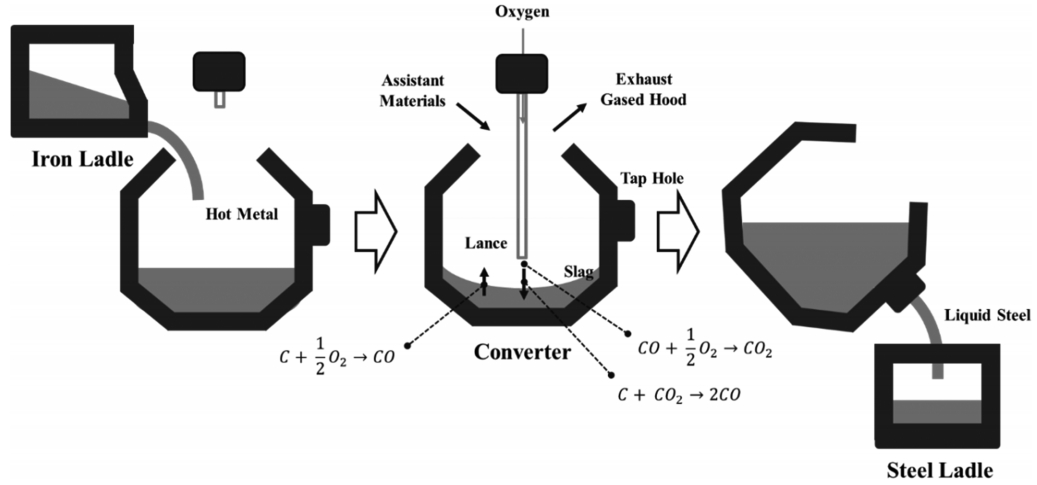
The hot transported metal contains significant amounts of impurities and cannot be used directly in the steelmaking process. To oxidize the carbon and other impurities and to adjust the metal’s composition, a converter is used in the BOF steelmaking process, as shown in Figure 1. The converter is a cylindrical steel shell lined with some refractory materials.
In the BOF process, the converter is tilted forward so that hot metal is charged. Relatively pure oxygen (more than 99.5%) is blown into the furnace through the vertical watercooled oxygen lance [18]. During this step, raw materials such as burnt-lime and iron ore are added into the furnace. The exothermic reactions of oxygen the elements such as Si, Mn and P remove the impurities, followed by the oxidation and elimination of carbon. During this step, oxygen is blown for about 20 min. The endpoint temperature, the carbon content and the compositions of other species are measured after blowing. If the measurements of the composition of C, P and Si or the endpoint temperature are not acceptable, additional oxygen is blown until the compositions of each species and the endpoint temperature satisfy the technical operation standards. If the compositions and the endpoint temperature meet the requirements, the liquid steel is tapped into the steel ladle. At that time, ferroalloys and the deoxidizers are thrown in the liquid steel to control the compositions.
The chemical reactions occurring in the furnace are exothermic reactions driven by high speed oxygen blowing with intense agitation. The main chemical reactions involved are as follows [19]:
The heat generated by the oxidation reaction of Si becomes the main source of temperature increase. In the carbon eliminating reactions, Fe reacts predominantly with oxygen to yield FeO which in turn is reacted with carbon. The temperature in the converter can be represented as [10]
where T0 is the temperature measured by the lance, Tr is the temperature raised by oxygen blowing, and Tc is the temperature decreased by the addition of the coolant.
2.2. Partial Least-Squares (PLS)
Partial least-squares (PLS) tries to identify so-called latent variables that capture the variance in the original data, and determines the maximum correlation between response variables Y and process variances X. PLS maximizes the covariance between the matrix of process variances X and the matrix of response variables Y. In PLS, the scaled matrices X and Y are decomposed into score vectors (t and u), loading vectors(p and q) and residual error matrices (E and F) as follows [20]:
where a is the number of latent variables. In the inner relation, the score vector t is regressed linearly according to the score vector u:
where b is the regression coefficient determined by the minimization of the residual h.
2.3. Artificial Neural Network (ANN)
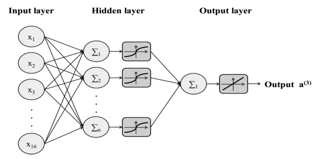
ANN, one of the most commonly used techniques in machine learning, consists of many simple neurons interconnected through a complex network. In a neuron, all signals from previous neurons are collected by weighted summation added by a bias. The output from the neuron is passed to the next neuron through an activation function [21].
The activation function used in the neuron can be represented as
where X denotes the summation of inputs fed into the neuron, xi is the value of the input i, wi is the weight on the input i, n is the number of input signals, and Y is the output from the neuron. Step, sign, sigmoid, and tanh functions are commonly used as the activation function. The basic activation functions such as step and sign functions generate 0, 1, or -1 as outputs. In general, sigmoid and tanh functions are most widely used. These functions convert input values ranging from –∞ to +∞ into the value lying between 0 and 1 or -1 and 1. These two functions can be readily adjusted to approximate a wide range of functions, including step and linear functions [22]. Figure 2 shows the prediction model based on ANN.
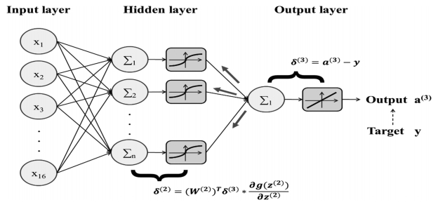
Typical multilayer neural networks consist of one input layer, multiple hidden layers and one output layer. In the learning process, the errors between the target values and the output values from the output layer are calculated. As shown in Figure 3, these errors are propagated in reverse to the input layer followed by the adjustment of weighting parameters. This kind of learning method is called a backpropagation learning algorithm.
The Backpropagation learning algorithm consists of the following two steps.
Step 1): perform the forward propagation operation by using the training data as in input to ANN. Calculate the differences between the predicted values and target values. These differences are regarded as errors which can be represented as
Step 2): Backpropagate these errors to the nodes within the ANN. Most machine learning algorithms employthe gradient descent method in which the objective function J(W) is continuously minimized. In the gradient descent method, the update procedure can be represented by
2.4. Least-Squares Support Vector Machine (LSSVM)
The support vector machine (SVM) can be considered a linear classifier which learns to minimize generalization errors. In SVM, the objective function for learning is defined using a margin to determine the optimal boundary among many linear decision boundaries [21]. The support vector is defined as data located at the nearest position to the decision boundary when the decision boundary classifying the learning data consisting of two classes is identified.
The Least-Squares Support Vector Machine (LSSVM) was proposed to replace SVM, which suffers from difficulty in solving Quadratic Programming (QP) problems. LSSVM is based on statistical learning using the least-squares scheme, and may be regarded as an alternative form of the SVM regression method [24]. The LSSVM optimization problem to estimate functions can be represented as Eq. (16) and (17):
Subject to
where ek denotes the error variable and φ is a normalized parameter representing the trade-off between the minimization of errors and the smoothness. The Lagrangian for the optimization problem can be defined as
where αk is the Lagrangian multiplier. The solution of the optimization problem yields the LSSVM model expressed by Eq. (19):
where K(x,xk) is the Kernel function [25].
3. ESTIMATION OF THE ENDPOINT TEMPERATURE
In the steelmaking process, accurate estimation of the endpoint temperature is very difficult because of the nonlinear relationships among the process parameters [9]. Various models have been proposed to predict the endpoint variable of molten steel for the purpose of reducing manufacturing cost and improving the quality of the steelmaking. If an accurate estimation of the endpoint temperature of the molten steel can be established, the amount of oxygen and coolant required to meet the target temperature (usually between 1,670 ℃ and 1,690 ℃) during the end-blow period in the steelmaking process can be accurately calculated prior to the operation.
The main chemical reactions that have significant effects on the endpoint temperature can be divided into heating and cooling reactions, as shown in Table 1.
Based on these chemical reactions, 16 input data to be used in the models were selected from the process data set, as shown in Table 2.
In this work, both the ANN and the LSSVM models were employed to estimate the endpoint temperature in the underlying steelmaking process. To obtain reliable estimation results it is imperative to select the appropriate choice of input variables that affect the endpoint temperature.
The input variables shown in Table 2 were used in the ANN and the LSSVM models to estimate the endpoint temperature. The results of the estimations were compared with those obtained from the PLS model, which is the classical estimation scheme, to evaluate the estimation performance.
4. RESULTS AND DISCUSSION
In this work, a total of 855 operational data sets were selected for training and model validation: 743 data sets were used to train the models and the remaining 112 data sets were used to validate the models. Table 3 shows the range of input conditions used for training in the models.
The estimation performance was evaluated using RMSE (Root Mean Square Error) defined as follows:
where ypred denotes predicted values, yactual are the actual values, and N is the number of data points used in the prediction.
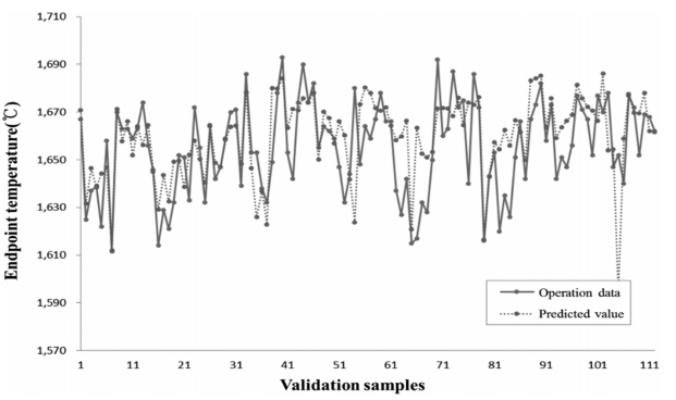
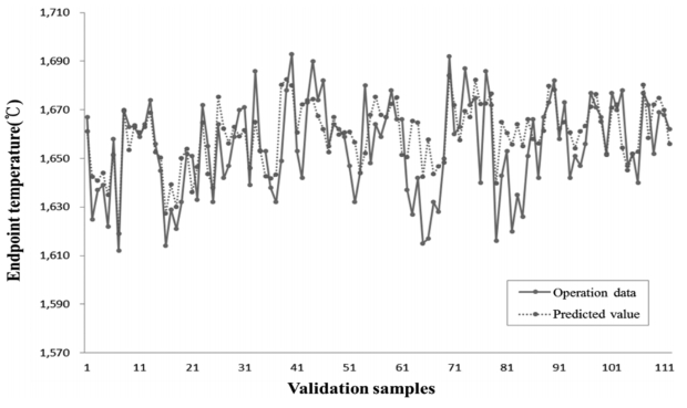
Figure 4 exhibits the results of the comparison between the operation data and the values predicted using the ANN model. The validation samples used on the x-axis mean the number of samples to validate the model.
The value of RMSE for the ANN model was 16.45. Figure 5 shows the results of the comparison between the actual values and the values predicted using the LSSVM model.
The value of RMSE for the LSSVM model was 14.29, which is a significant improvement over the estimation based on the ANN model. For additional model comparison, the classical PLS model was employed as the base case. The prediction results of the PLS model are displayed in Figure 6.
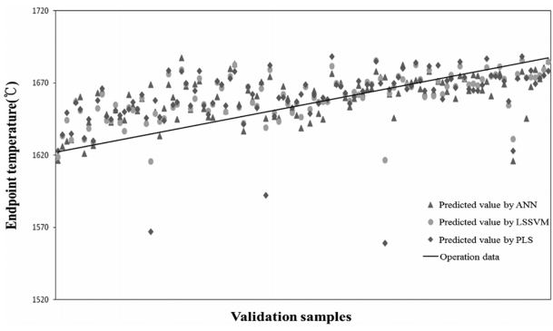
The value of RMSE for the PLS model was 21.24, which is much larger than those for the ANN and the LSSVM models. The values predicted by the three models with the trend line of the operation data are displayed in Figure 7.
The maximum deviation was utilized to carry out a comparative analysis of the estimation performance [3]. The maximum deviation is defined as the percent of the predicted values that lie within a range of ±15 ℃ of the measured endpoint temperatures. Table 4 shows the maximum deviations of the three estimation models.
As can be seen in Table 4, the LSSVM model shows the best estimation performance compared with the remaining models, followed by the ANN model.
In the analyses so far, all 16 initial input parameters have been used to calculate the value of RMSE for each model. However, some of the input parameters had negligible or little effect on the endpoint temperature estimation performance. To investigate which they were, the value of RMSE was sequentially calculated with one input parameter omitted, using the remaining input parameters. If the calculated RMSE was larger than the previous value, the omitted input parameter was considered to be an essential parameter with a significant contribution to the endpoint temperature. On the other hand, if the calculated RMSE turned out to be smaller than previous value, the omitted input parameter was considered to have a negligible effect on the endpoint temperature, and was excluded to improve the estimation performance. Using this sequential selection process, finally only the essential input parameters remained, after excluding parameters that had negligible effect on estimation performance. Then the value of RMSE was calculated for each model using the new selected input data sets.
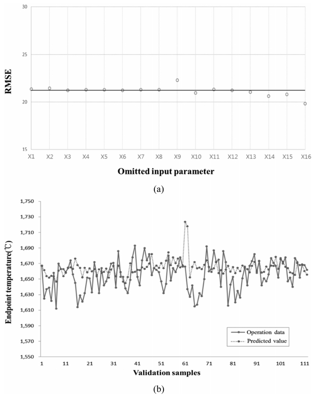
In the ANN model, each input parameter was sequentially omitted from the 16 input parameters, and the RMSE was then recalculated for the estimation based on the remaining input parameters. As shown in Figure 8(a), some RMSEs with one input parameter omitted were lower than previous result obtained using all 16 input parameters. Accordingly, X1, X2, X4, X5, X6 and X7 were considered to be negligible input parameters that had little effect on the estimation performance. The ANN model was constructed again after these input parameters were excluded, and the RMSE was recalculated again using the remaining 10 input parameters. Figure 8(b) shows the results of the comparison between the operation data and the predicted values for the ANN model. The recalculated RMSE is 16.36, which is less than the 16.45 obtained using all 16 input parameters.
As shown previously, the initial RMSE for the LSSVM model using all 16 input parameters was 14.29. As was done with the ANN model, the RMSE was recalculated after one input parameter was sequentially omitted and the estimation was based on the remaining input parameters. As shown in Figure 9(a), some RMSEs with one input parameter omitted sequentially were lower than the base value, 14.29. X9, X14 and X15 were accordingly considered to be negligible input parameters which had a negative effect on the estimation performance. The LSSVM model was then recalculated using the remaining 13 input parameters. Figure 9(b) shows the results of the comparison between the operation data and predicted values using the LSSVM model. The recalculated RMSE was 13.21, which is less than the base case, 14.29. This confirms that the RMSE for the LSSVM model is reduced through the sequential input selection process.
Finally, the sequential input selection process was also applied to the PLS model, and RMSE was recalculated for the estimation. As shown in Figure 10(a), the RMSEs with omitted input parameters X10, X13, X14, X15 and X16 were lower than the base value, which was 21.24. The PLS model was constructed again after these parameters were excluded, and RMSE was recalculated using the remaining 11 input parameters. Figure 10(b) shows the results of the comparison between the operation data and the predicted values using the PLS model. The recalculated RMSE was 22.14, which is larger than base value of 21.24. We can see that the sequential input selection process has no positive effect on the estimation performance of the PLS model.
Table 5 shows the input parameters obtained from the sequential input selection process, and Table 6 shows the resultant RMSEs using all 16 input parameters and the resultant RMSEs using remaining input parameters after the sequential input selection process for the three models.
As demonstrated in Table 5, the selected input parameters obtained by the sequential input selection processes are different for each model. This is due to the different effects of various data on each model, based on statistical learning. The RMSE values used in the sequential input selection process are different for each model. Therefore, as shown in Figs 8-10, some input parameters were discarded due to their small effect on the RMSE values, and the remaining input parameters are therefore different in each model. It is difficult to identify interactions among input parameters in the sequential analysis method. In order to take interactions among input variables into account, the correlation analysis method or variable selection method widely used in big data mining schemes should be applied. But the primary purpose of this study was to improve estimation accuracy, and it was found that the sequential analysis method is very efficient for that purpose. As can be seen in Table 6, it is confirmed that the LSSVM model with 13 input parameters obtained from the sequential input selection process exhibited the best estimation performance among the three estimation models considered in this study.
5. CONCLUSIONS
The ANN model and the LSSVM model were used to predict the endpoint temperature of molten steel produced in the steel making process. The classical PLS model was used as a base case for model comparison. The estimation performance was evaluated using RMSE values and when all 16 input parameters were used, the RMSE value of the LSSVM model was 14.29 and that of the ANN as 16.45. The RMSE of the PLS model was 21.24, the poorest estimation performance of the three models. The RMSE values of the three models were then recalculated using input parameters obtained from the sequential input selection process. As a result, the RMSE value of the LSSVM model was 13.21 and ANN was 16.36. From the model comparison, the LSSVM model with the 13 input parameters obtained from the sequential selection process had the best estimation performance, compared to the ANN and PLS models. The LSSVM model is expected to be used to accurately calculate the amounts of oxygen and coolant required to achieve the target temperature during the end-blow period in the steel making process.